Perfect Competition
- Detalii
- Categorie: Microeconomics
- Accesări: 11,070
Perfect Competition
So far, we have discussed how the consumers make their decisions, and what the producers’ production possibilities and cost of production look like. The consumers often take prices as given and choose quantities based on the prices. The question is how prices arise. One factor is, of course, the cost of production.
The price cannot be below the cost, at least not in the long run. The price is, however, very dependent on the structure of the market. Among the most important questions one can ask about the market structure are:
- The degree of concentration of buyers and sellers. Do we have many, a few, or one?
- The degree of product differentiation. Are the products identical to
- each other, or how different are they from each other? (See Chapter 15, on monopolistic competition.)
- Are there any barriers to entry in the market? (See Chapter 11 on monopoly)
The answers to these questions largely determine which kind of market we get, and this, in turn, largely determines the price. In this chapter, we will look at one type of market, a perfectly competitive market. In later chapters, we will look at other market forms.
Conditions for Perfect Competition
For a market to be perfectly competitive, it has to fulfill the following conditions:
- All agents are price takers. No single buyer or seller can affect the price of the good. Everyone takes the price as given, and, depending on the price, decides about quantity. This condition will be true if there are many small buyers and sellers.
- Homogenous products . Each seller’s products are identical to every other seller’s products. Furthermore, there are no extra costs, such as transportation costs, for some sellers. The buyers are therefore neutral between different sellers.
- All factors of production are completely variable. There are no barriers to entry for new firms or barriers to leave for existing firms.
- All buyers and sellers have complete information about existing alternatives in the market.
- There are no agreements to collude in the market. For instance, the sellers cannot form a cartel.
These conditions are hard to satisfy and few, if any, real markets do that. Even so, the model is very informative and delivers several interesting results. Furthermore, many economists are highly in favor of competition and some of the most important reasons for that will be revealed as we use this model
Profit Maximizing Production in the Short Run
The goal of an individual firm is to maximize its profit, i.e. the difference between revenues and costs. In the short run, it does that under the restriction that it cannot change the amount of capital. We will now study the short-run production in a diagram. In the upper part of the diagram in Figure 9.1, we have drawn the total cost, TC, total revenue, TR, and the profit, π = TR - TC. Since the firm cannot influence the price in a perfectly competitive market, TR will simply be a straight line with a slope equal to p (the price). This is since each additional unit of the good it sells will yield an income of p. The shape of TC is often more complicated (see Section 8.1).
The goal is to maximize the profit, which in the graph occurs at a quantity of q = 78 units, where the profit is 41. (This is the point where π reaches its maximum.) As profit is the difference between revenues and costs, the difference between TR and TC is at a maximum here: 172 - 131 = 41.
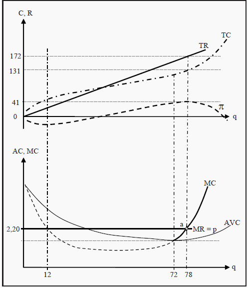
Figure 9.1: Profit Maximization under Perfect Competition
The price, p, the marginal cost, MC, and the average variable cost, AVC. MR corresponds to the slope of TR, which we argued must be equal to p. In other words, if we sell one more unit of the good, we receive an additional income equal to the price, p. Therefore, MR is equal to p. In point a, the MC curve intersects the MR curve.
This is a condition for profit maximization. To see why, think about what would happen if we sold one unit more or one unit less than 78. If we had produced and sold one unit more, we would have incurred a cost of MC, but we had only received an income of MR. And MR < MC, so we had reduced profit.
Conversely, if we had produced one unit less, we would have saved the production cost of that unit, MC, but we would also have lost the revenue from selling it. Moreover, to the left of 78, MR > MC, so we had reduced profit that way as well. Therefore, 78 is indeed the best choice we can make. The condition for profit maximization is:
MR (q*) = MC (q*)
that, at the quantity 78 in the figure, TR and TC have the same slope. That is the same thing as MR = MC.
Strategy to Find the Optimal Short-Run Quantity
We can summarize the strategy for finding the point where the firm maximizes its short-run profit in a few steps:
- Find the point where MC = MR and where the MC curve is increasing.
- Is that point above (or equal to) AVC, i.e. is p = MR >AVC? In that case, choose to produce the corresponding quantity.
- In the opposite case, i.e. if p = MR < AVC, choose to produce nothing at all; q = 0. The condition p = MR < AVC is called the shutdown condition.
Note that (as in the first bullet point) the MC curve must be increasing. In Figure 9.1, we can see that the MC curve also intersects the MR curve at the quantity q = 12, but there the MC curve is decreasing. That point instead maximizes the loss!
Also, note for bullet points 2 and 3, the reasoning behind the condition MR >AVC: Since we are looking at the short run, the fixed cost, FC, cannot be changed. The firm can always choose to produce nothing. If it does so, it receives no revenues and incurs no variable costs, but it will still incur the total fixed cost, FC.
Total profit will then be a loss of -FC. This means that the firm will choose to produce as long as it can at least recover some of that loss. Moreover, the firm will do so as long as the price, and therefore MR, is larger than or as large as AVC.
In the short run, the firm can consequently accept to produce at a (small) loss, since the loss will be smaller than if one chooses to shut down production completely. If instead MR < AVC, the revenues from additional units sold cannot even cover the average variable cost of producing them. Then it is better to shut down.
The Firm’s Short-Run Supply Curve
What happens if the market price changes? Then MR changes, and the point of intersection between MR and MC also changes. The firm will then choose to produce the quantity that corresponds to the new point of intersection, so the quantity supplied follows the MC curve as the price changes.
However, this is only true as long as the price is higher than AVC. To see why, look at the shutdown condition above again. Suppose the market price falls to the point where the MC curve intersects the AVC curve, i.e. at the quantity q = 72 in the figure. At that point, MR = p = MC = AVC and the profit becomes q*(p - AVC) - FC = 72*0 - FC = -FC. Note that p – AVC is what the firm gets paid in excess of average variable cost for each unit it sells; q*(p - AVC) is then what it gets paid in excess of average variable cost for all units it sells; finally, subtracting FC yields what it gets paid in excess of all costs (= profit).
The loss is consequently as large as if we choose to produce nothing at all. If the price falls even more, the losses increase and it is better to produce nothing. The conclusion of this is that, the firm’s short-run supply curve is the part of the MC curve that lies above AVC, i.e. the part that is drawn with a full line in the lower part of Figure 9.1.
The Market’s Short-Run Supply Curve
The market is the sum of all individual firms. We get the market’s supply curve by summing all individual firms’ supply curves horizontally. Compare to the method used in Section 4.2.
Short-Run Equilibrium
In Figure 9.2, we have summarized the equilibrium in the market and the equilibrium for an individual representative firm. To the right in the figure, we have the individual firm’s MC-, ATC-, and AVC curves. The short-run supply curve of the firm is the part of the MC curve that is above AVC. For prices below pmin, there is consequently no supply at all. If we sum all firms’ supply curves, we get the market’s supply curve, S, to the left in the figure. (∑(MC) means "the sum of all MC curves.")
In the market, supply meets demand, D, and an equilibrium price, p*, and an equilibrium quantity, Q*, arise. p* is the price that the individual firm receives for each unit of the good it sells. Since there are a large number of firms, no individual firm can charge a higher price than p*. If some firm did, the consumers would choose one of its competitors instead.
The MR curve of an individual firm is consequently horizontal and equal to the price, p*. The firm chooses to produce the quantity q*, as this quantity makes MC = MR and, consequently, maximizes profit.
In the short run, a firm in a perfectly competitive market can make a profit. In Figure 9.2, the profit corresponds to the grey rectangle on the right-hand side. To see that this is the profit, note that in a perfectly competitive market AR (Average Revenue) is as large as MR is, since the firm is paid the same amount for each unit sold. Furthermore, q*AR = TR and q*ATC = TC. Profit is then π = TR - TC. To summarize, we have that
π = TR -TC = q * AR - q * ATC = q *(MR – ATC)
The right-hand side of this expression corresponds to the grey rectangle in Figure 9.2. With the example we used before, we get that π = 78*(2.20 - 131/78) = 41.
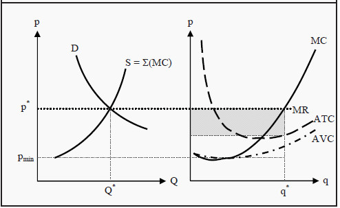
Figure 9.2: Short-Run Equilibrium for the Market and an Individual Firm
Long-Run Production
The firm in Figure 9.2 makes a short-run profit. However, what happens in the long run? There are three different possibilities: The firm could make a profit, make a loss, or break even. The first is called excess profit or supernormal profit, and the last is called normal profit. No firm can allow itself to make a long-run loss.
In the long run, a firm in a perfectly competitive market will make normal profits, i.e. break even. To see that, look at Figure 9.3. Here, we have the same initial situation as in Figure 9.2. Since the firm makes a profit, this market will attract new firms.
Moreover, since there are no barriers to entry, new firms will producers establish themselves in the market, larger and larger quantities will be supplied at each given price, and the market supply curve will shift to the right, from S1 towards S2. Consequently, the price will be pushed down, from p1 * towards p2 *. For the individual firm, the decrease in the price means that it will reduce the quantity it produces, from q1* to q2 *.
Remember that the firm chooses to produce the quantity where MR (= p) = MC. This process, with new firms and reductions in prices, continues as long as there are any profits to be made in the market. When the price reaches p2*, and the firm produces the quantity q2*, we are exactly at the point where the MC curve intersects the ATC curve. In the previous section, we showed that π = q*(MR - ATC), and a quick look at that expression gives that if MR = ATC then the profit must be zero, regardless of the quantity produced.
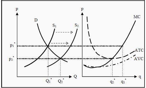
Figure 9.3: Long-Run Equilibrium for the Market and an Individual Firm
When the price has reached p2*, there are no longer any excess profits to be made in the market. No more firms establish themselves and the downward push on the price stops. The market is then in long-run equilibrium. Note that the individual firm reduces the quantity it produces, while the total quantity produced in the market increases. The reason for this is that enough many new firms establish themselves to counterweight the reduction in production for the individual firm.
In the short run, we can also have the opposite case: The individual firms can make short-run losses. That will cause some firms to leave the market in the long run and total supply decreases, which causes the equilibrium price to rise. That process will continue until no firm makes a loss, and the endpoint of that process is the same as before: p2* and Q2*.
Many people find the result that firms in a perfectly competitive market make zero profits, hard to accept. Remember, however, that by a cost in this context we mean opportunity cost. Therefore, the revenues are as large as the opportunity costs. In the opportunity costs, we include what the firm loses by not investing in the best alternative. If the best alternative is a very good one, the situation here will also be good for the firm. Also, remember that, there are very few real-life examples of a perfectly competitive market, so it might be difficult to have a good intuition for this result.
The Long-Run Supply Curve
For the individual firm, the long-run supply curve is found in exactly the same way as the short-run, only with long-run marginal cost, LRMC, and average cost, LRAC, instead. The supply curve is, consequently, that part of LRMC that lies above LRAC.
When it comes to the whole market’s long-run supply curve, the situation is much more complicated. Remember that, for the short run we found the market’s supply by summing up all existing firms’ supply curves. That was possible because in the short run the number of producers is constant. This is not the case in the long run. If the price changes, then, in the long run, the number of producers also changes.
The market long-run supply curve instead depends on how the cost of production changes with the size of production for the whole market.
- Constant production cost. If it is possible to establish new firms and they will have exactly the same cost of production as existing firms, then the industry has constant costs. If this is the case, the long-run supply curve will be a horizontal line. The reason for that is that, if the price would be higher at some quantity, new firms would establish themselves. Moreover, the cost for the new firms is the same as for the old firms, so this will push down the price to the marginal cost.
- Increasing production cost. If it costs more and more to produce more units, the industry has increased costs. To produce more, firms have to increase the price per unit. The supply curve will therefore slope upwards (i.e. in the opposite direction of any of the supply curves in this book).
- Decreasing production cost. In the opposite case, if it costs less and less to produce more units, the supply curve will slope downwards.
Properties of the Equilibrium of a Perfectly Competitive Market
Several central properties of the perfectly competitive market equilibrium deserve to be pointed out. These properties are the primary reasons why many economists (normatively) view a high level of competition as a good thing.
The equilibrium is efficient. The market price will be at the same level as the long-run average cost of production. There is consequently no other way to produce the same quantity of goods that is cheaper.
There is, in other words, no waste of resources.
- All firms have normal profits, i.e. no profits. The consumers, consequently, pay only what the production costs.
- Total utility is maximized.
Note also that these results, that are positive for society, are achieved without any form of central planning or ruling. This phenomenon, that the resources automatically are allocated such that these results are achieved, is often called the invisible hand.
However, remember that to reach these results, we have assumed a perfectly competitive market, i.e. that all the assumptions in Section 9.2 are satisfied. We will soon look at other markets forms.
Market Interventions and Welfare Effects
There are many different opinions about what welfare is. When one talk of welfare effects in microeconomics, then it is most often about how much utility different groups of people get from different allocations of goods. Usually, welfare analyses separate between producers and consumers, and make the following distinctions:
Consumer surplus ( CS ). The consumers have a certain valuation of a good and pay a certain price to get it. The consumer surplus consists of the difference between how high their valuation is and how much
they pay. In Figure 10.1, this corresponds to the triangular area labeled CS, i.e. the area between the demand curve and the price.
We can get an intuition of why this area is interesting in the following way. Suppose we are the customer with the highest valuation of the good. We would then be the customer that is willing to pay the highest price for it. In other words, we are the customer who defines the left-most point on the demand curve, D. If the price were so high that only one unit was sold, we would be the buyer. However, at the equilibrium, we do not have to pay that high price. We only have to pay p*.
That means we get a surplus, as compared to what we are willing to pay, corresponding to the difference between the point on D and p*. If we apply the same reasoning to the consumer with the second-highest valuation, and so forth for all consumers who buy the good, we get the result that the total consumer surplus corresponds to the area CS in the figure.
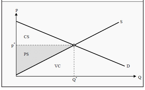
Figure 10.1: Consumer and Producer Surplus
Producer surplus ( PS ) is the difference between what the producers are paid for a good and the lowest price at which they would have supplied it (i.e. the marginal cost of production). In Figure 10.1, this corresponds to the triangular area labeled PS, i.e. the area between the price and the supply curve. The reasoning behind why this area is interesting parallels the one for the consumers.
Social surplus is the sum of consumer and producer surplus: CS + PS. One may note that PS is directly related to profit. The area below the supply curve, S, i.e. the triangle labeled VC, corresponds to the variable cost of production. The producers’ total revenue, TR, is the price times the quantity sold. From the figure, we see that p* *Q* = TR = PS + VC
Furthermore, we know that profit is revenues minus costs. We can therefore get an expression for the profit:
π= TR – ЕС
=TR –(VC-FC )
=(PS+VC) – (VC-FC)
=PS-FC
In the short run, profit consequently equals PS minus fixed costs. In the long run, there are no fixed costs, and PS and profit are equal to each other.
Welfare Analysis
CS, PS, and social surplus are often used to evaluate the effects of market interventions.
Such an analysis is called a welfare analysis.
Let us use an earlier example. In Section 2.4.2, we studied the effect of a maximum price in a perfectly competitive market. With the help of Figure 10.2, we can now compare the social surplus with and without the maximum price.
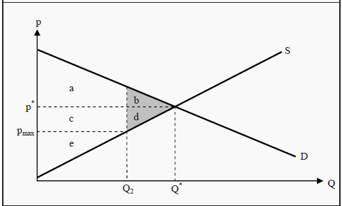
Figure 10.2: Social Effects of a Maximum Price
The maximum price decreases the market price from p* to pmax and the quantity from Q* to Q2. Before the maximum price was introduced, CS = a + b, PS = c + d + e, and the social surplus equaled a + b + c + d + e. After the maximum price is introduced, CS = a + c, PS = e, and the social surplus is a + c + e. The producers have consequently lost c + d, and the total welfare has decreased by b + d. The consumers have lost b but gained c.
Whether the consumers are better or worse off depends on if the area c is larger or smaller than b. However, a social surplus is always diminished by introducing a maximum price in a perfectly competitive market. The amount of social surplus that is lost, b + d, is called the deadweight loss.